Signal integrity

The tool

1. Choose a topology at the top left, or switch to Schematic and draw the net yourself.
2. Choose the driver and receiver models: one of the built-in generic models, or your own IBIS file (Load IBIS file…).
3. Change any value by typing it (with units, such as 1.2 ns or 33), by dragging its slider, or with the mouse wheel over the box (hold Shift for bigger steps).
4. The scope re-simulates at once. Undo and redo with Ctrl+Z and Ctrl+Shift+Z.

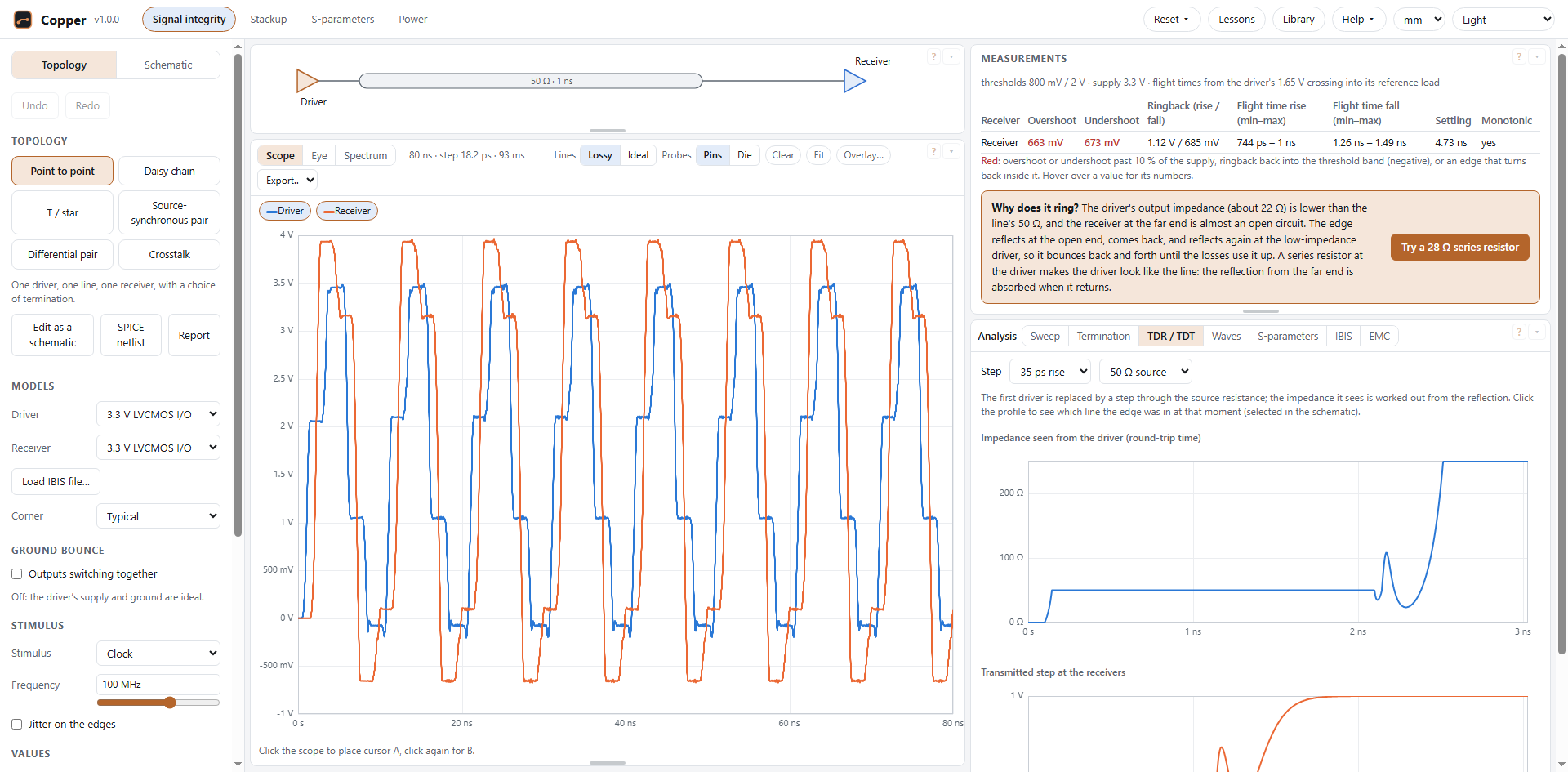
The built-in models are generic examples made for this tool (3.3 V LVCMOS, 1.8 V CMOS, a 1.2 V DDR-like I/O and a fast 2.5 V output). They are not models of real devices.

Topologies and values

• Point to point: one driver, one line, one receiver.
• Daisy chain: a trunk from the driver, then two to eight receivers along the bus, each on its own stub.
• T / star: a trunk to a hub, then a branch to each of two to six receivers.
• Source-synchronous pair: a clock net and a data net (PRBS) side by side; Copper reports setup and hold at the receivers.
• Differential pair: a differential driver, a coupled pair on the stackup and a receiver with a resistor across its pins (see Differential pairs).
• Crosstalk: an aggressor and a quiet victim side by side on the stackup (see Coupled lines and crosstalk).

Lines are lossless and described by their impedance Z0 and delay. Terminations: series (a resistor at the driver), parallel (a resistor at the far end, to ground or to a voltage), Thevenin (a resistor to the supply and one to ground), AC (a resistor in series with a capacitor to ground). Load C adds a capacitor at each receiver.

The stimulus is a clock by default, so both edges show; a single edge or a PRBS pattern can be chosen instead. The source-synchronous pair drives its own clock (at half the bit rate, edges mid-bit) and data.

Schematics

The Topology / Schematic switch at the top left changes how you set up the net. In Schematic you draw it: any part, any wiring. Each ready-made topology opens as a schematic (Edit as a schematic, or Start from a topology), so it can be the starting point of your own net. The scope runs on every change, as with the topologies.

• Add a part with the buttons under Parts or from the command list (Ctrl+K): drivers and receivers (IBIS), resistors, capacitors, inductors, lines and coupled lines, ground, supplies, voltage and current sources, ports, and the parts under More parts (S-parameter blocks, vias, beads, connectors, packages, cables).
• Wire by dragging from a pin (or from a wire) to where the wire should end. Copper draws it square and places its corners where they join nothing else. Wires join at their ends and where an end meets the middle of another wire (a dot shows it); wires that only cross are not joined.
• Move parts by dragging them; their wires follow, each drawn again from the nearest junction or pin so corners never pile up. To move a wire, drag it sideways (the wires at its ends stretch to follow; a move that would join or part a net is refused); a click selects it, and Alt+drag from a wire starts a new wire there. T (or Tidy the wires in the command list) draws every wire again, square and as short as it can, with the nets exactly as they were. Select several with Shift+click or by dragging a box on the empty grid. R rotates, Delete deletes, Escape clears the selection, F fits the drawing in view.
• Notes: N (or Note in the palette) puts text on the drawing; double-click a note to edit it (Shift+Enter for a new line; an empty note is deleted). Notes have no electrical meaning; they are kept with the design.
• Values: double-click a value on the drawing to type it, or scroll over it (Shift for bigger steps). The selected part's values, model and role are also on the left.
• Probes: Alt+click a pin to show it on the scope (again to remove it), or tick Show on the scope. Hover any pin or wire to see its waveform from the last run.
• Colours: after a run, the net at each receiver on the scope turns green when it measures well, amber when overshoot or undershoot passes 5 % of the supply, and red past 10 %, with ringback into the threshold band or a non-monotonic edge.
• Zoom with the mouse wheel; pan with the middle button, Space+drag or Shift+wheel. A pin drawn with a red ring is not connected to anything. Undo and redo with Ctrl+Z and Ctrl+Shift+Z.

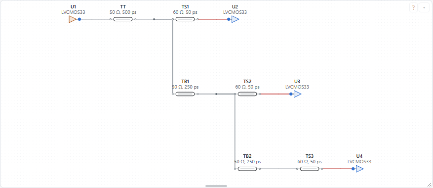
The circuit's stimulus and corner are under Simulation. A design can also hold drivers with their own stimulus (the source-synchronous pair's clock and data). Flight times are taken from the driver nearest to each receiver along its net.

Designs, files and links

• Every schematic is a design, kept in this browser as you work: Designs in this browser lists them to open again or delete. Rename the open one in Name; New starts an empty one.
• Save file writes the design as a file, with the IBIS files you loaded yourself inside it, so it opens complete on another computer (Open file…). Circuit files without a drawing open too: Copper draws them.
• Copy link puts the whole design in a link. The design travels in the part of the address after the #, which browsers do not send to the server. Models are named in the link but not carried: built-in models load by themselves, and the person who opens the link is asked for any others.
• SPICE netlist (in a schematic, or beside Edit as a schematic for a topology) saves the circuit for a SPICE simulator: resistors, capacitors, inductors, sources (following the stimulus, as piecewise-linear sources), supplies, ports (their resistance), lines as lossless T elements (each line's loss is noted beside it), and coupled lines exactly, by their modes (one T line per mode, joined to the conductors by controlled sources). Vias, beads, connectors, packages and cables are written as the parts they run as. IBIS buffers and S-parameter blocks have no SPICE form here: they are listed at the top of the file with their nodes, to add your own models there.
• Report saves the design as one web page, to keep or print: the drawing, its parts, the settings, the lines as they ran (impedance, delay, loss), the scope and the measurements.

Stimulus: patterns, coding and jitter

Under Stimulus (or Simulation in a schematic): a single edge, a clock (its frequency and duty cycle), or a pattern at a bit rate, either a PRBS (7, 9, 11, 15, 23 or 31) or bits you type.

• Coding puts a line code over a PRBS: 8b/10b (each byte as ten bits, kept DC-balanced by its running disparity) or 64b/66b (64 bits scrambled by 1 + x^39 + x^58 behind a two-bit sync header). Coded data has fewer long runs of one value than the raw PRBS, so its eye closes less from the line's slow tail.
• Jitter on the edges moves every edge of a clock or pattern: random (Gaussian, its rms; the same sequence on every run, so results repeat), sinusoidal (its peak and frequency), and duty-cycle distortion (rising edges late and falling edges early by half of it). Each edge moves by at most 0.45 of a unit interval.

IBIS models and corners

Copper reads IBIS files: the I-V tables, the clamps, C_comp, the package, and the switching behaviour from the V-t waveforms (or from [Ramp] when a model has none). Keywords outside that set (for example power-aware or algorithmic models) are listed when the file is loaded and are not used.

Corners: slow-weak uses each table's min column, fast-strong the max column; C_comp and the package take their larger value with slow and the smaller with fast. The package is a resistance and inductance in series, with half of its capacitance at each end.

The scope

• Probes sit at the driver and at every receiver. Probes: Pins | Die switches between the package pins and the buffers inside the packages.
• Earlier results fade behind the newest (afterglow), so a change reads as movement. Clear wipes them.
• Click the scope to place cursor A, click again for B: the table below gives each probe's voltage at both and the differences. Click a probe's chip to hide or show it (with every probe hidden, Show all brings them back). Drag a box to zoom, Shift+drag (or drag with the right button) to pan, Ctrl+wheel to zoom around the pointer; Fit (on the scope's bar) or a double-click shows all of it again.
• Scope / Eye switches the card to eye diagrams of the probes shown (see Analysis).
• Spectrum shows each probe's spectrum in dBµV over a logarithmic frequency axis: the run after its first tenth (once the net has settled into its pattern), with a Hann window, scaled so a sine of amplitude A reads A.

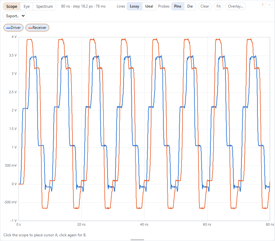
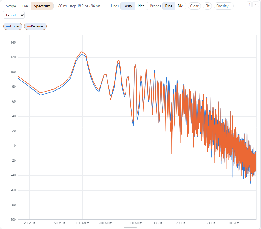
Export… in the scope's header saves what it shows: an image (PNG, or SVG to edit), with its title and legend, or the waveforms as data (CSV, one time column and one column per trace).

Overlay… lays waveforms from a CSV file over the scope, dashed: a time column, then one or more voltage columns; a header row is optional, and units in it are read ("Time (ns)", "V(out) (mV)"). N overlaid × takes them away. In a schematic, select a resistor, capacitor, inductor, line or source and tick Show its current: the currents get a plot of their own (amperes) under the scope.

Measurements

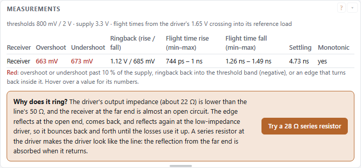
For every receiver, with the receiver model's thresholds Vinl and Vinh and its supply. A value in red is one to look at: overshoot or undershoot past 10 % of the supply, ringback back into the threshold band (negative), or an edge that turns back inside it; hover over it for its numbers, and a line under the table says the same.

• Overshoot: how far the signal goes above the supply. Undershoot: how far it goes below ground. Values over a tenth of the supply are shown in red.
• Ringback: after a rising edge has crossed Vinh and peaked, the closest it comes back down to Vinh (and the mirror image against Vinl for falling edges). A negative value means it rang back into the threshold band, where the receiver may switch twice.
• Flight time: when the receiver crosses its thresholds, measured from when the driver alone, into its own reference load (Rref, Cref to Vref), crosses Vmeas. The minimum uses the first crossing of the nearer threshold, the maximum the last crossing of the farther one.
• Settling: from the first edge until the signal stays within 5 % of its swing of its final level.
• Monotonic: whether the signal moves one way only while it is inside the threshold band.

When a receiver's voltage goes beyond what its model's clamp tables cover (the GND clamp against ground, the POWER clamp against the supply), a note under the table says so: there the clamp current is extended in a straight line, not measured, so the overshoot the model allows is a guess.

Why does it ring?

A driver is a low impedance (often 15–40 Ω), a line is typically 40–60 Ω, and a receiver input is almost an open circuit. The edge travels down the line, reflects at the open far end (doubling), returns, and reflects again at the low-impedance driver, now inverted. So it bounces back and forth, and the receiver sees overshoot and ringing until the losses use it up.

The cures make one end match the line. A series resistor at the driver, about Z0 minus the driver's own impedance, absorbs the reflection when it returns: the receiver then sees one clean step. A parallel or Thevenin termination at the far end absorbs the edge on arrival, at the cost of DC current. When the net rings and has no termination, the measurements offer a series resistor to try, with one click; the Termination view under Analysis compares every kind.

Ground bounce

A chip's outputs share its supply and ground pins. When many switch at once, their current changes fast through the inductance of those pins, their bond wires and vias, and the chip's own ground and supply move against the board's: ground bounce (or simultaneous switching noise). A quiet output of the same chip moves with them, and an edge of a switching one slows and grows a step.

Under Ground bounce (below the models in a topology, or on a selected driver in a schematic) tick Outputs switching together and give:

• Outputs: how many outputs like this one switch at the same instant, the same way, each into a net like this one (8 to start).
• Ground L and Supply L: the inductance of the shared ground path and of the shared supply path, all their pins, bond wires and vias together (1 nH each to start: about two to four pins of a small package).
• Die C: the chip's own capacitance between its supply and ground (0: none). It supplies the first part of each edge's current and calms the bounce.

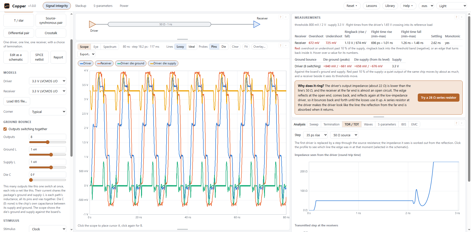
The driver's pull-up and power clamp then work against the die's supply, its pull-down and ground clamp against the die's ground, and those connect to the board through the shared paths. As every output carries the same current, Copper simulates this one with the whole group's current through the paths: the same answer as simulating them all, and no slower. The scope gains die ground and die supply traces (against the board's ground), and Measurements gives their peaks either way, red past 10 % of the supply. To see how the bounce grows with the count, sweep Outputs under Analysis and watch the die ground.

Differential drivers are left out: the two halves of a pair switch opposite ways and most of their current cancels in the shared paths.

The die nodes' waves are checked against an independent solution of the same circuit, within 0.02 % of their swing.

Analysis: eye, sweep, termination, TDR, waves, S-parameters, IBIS, EMC

Under the scope, the Analysis card has views that run the net many times or look at it another way. They use the net as it is on the scope, in the current mode (topology or schematic), with the Lines switch as set. The card opens on TDR / TDT. TDR / TDT, Waves and EMC take one run each: like the scope they are worked out as soon as their tab opens and again, once, after every change. The sweep and the termination advisor take many runs and the S-parameters are set up first, so those start with their button.

Eye

Eye on the scope card folds each probe's waveform into two unit intervals, centred on the eye, and shades how often the signal passes each point, like a persistence display. The unit interval is a bit of a PRBS pattern or half a period of a clock (an eye needs one of those as the stimulus). Under each eye: its height and width, the jitter of its crossings, and for a receiver a mask from its thresholds (Vinl to Vinh, or ± the differential threshold) over the middle fifth of the interval, red when the signal crosses it. Earlier runs fade under the newest one.

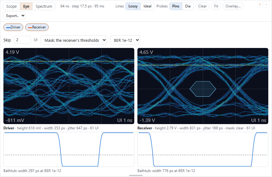
Above the eyes: how many unit intervals to skip at the start (while the net settles), the mask (the receiver's thresholds, your own width and height, or none) and an error rate. Under each eye a bathtub: the error rate across the unit interval from the dual-Dirac model, its deterministic part from the spread of the simulated crossings and its random part from the random jitter on the stimulus; it gives the eye's width at the error rate chosen. Without random jitter on the stimulus the bathtub has straight walls.

Sweep

Up to three variables at once: any value on the left, a stackup value (a layer's thickness, a dielectric's Dk or Df, the solder mask, the etch factor) or the corner, each over a range of 1 to 10 points (linear or logarithmic). Every combination is a case (the first variable outermost, at most 200), run in turn and measured at the watched probe as the measurement table measures a receiver: highest and lowest, overshoot and undershoot, the worst ringback (negative: back into the threshold band), the first crossing of the threshold, settling and monotonic edges. Click a heading to sort, a row to pick out its trace; Use these values puts a case's values on the sidebar. Table (CSV) and Waveforms (CSV) save the results; Stop ends a long sweep early.

Statistical (the Kind switch) draws every variable at random instead, for 20 to 500 cases: each one anywhere in its range (Uniform) or around the middle of it, with the range as ±3σ (Normal, the way tolerances usually spread; a value past the range is drawn again), and the corner at random. A case fails when a value turns red (overshoot or undershoot past 10 % of the supply, ringback into the threshold band, an edge that turns back). The summary gives how many failed, with the range the true failure rate lies in with 95 % confidence (from 20 cases with none failing: up to about 16 %; more cases narrow it), and each measurement's lowest, mean, highest and standard deviation. Each run uses a new seed, shown with the results.

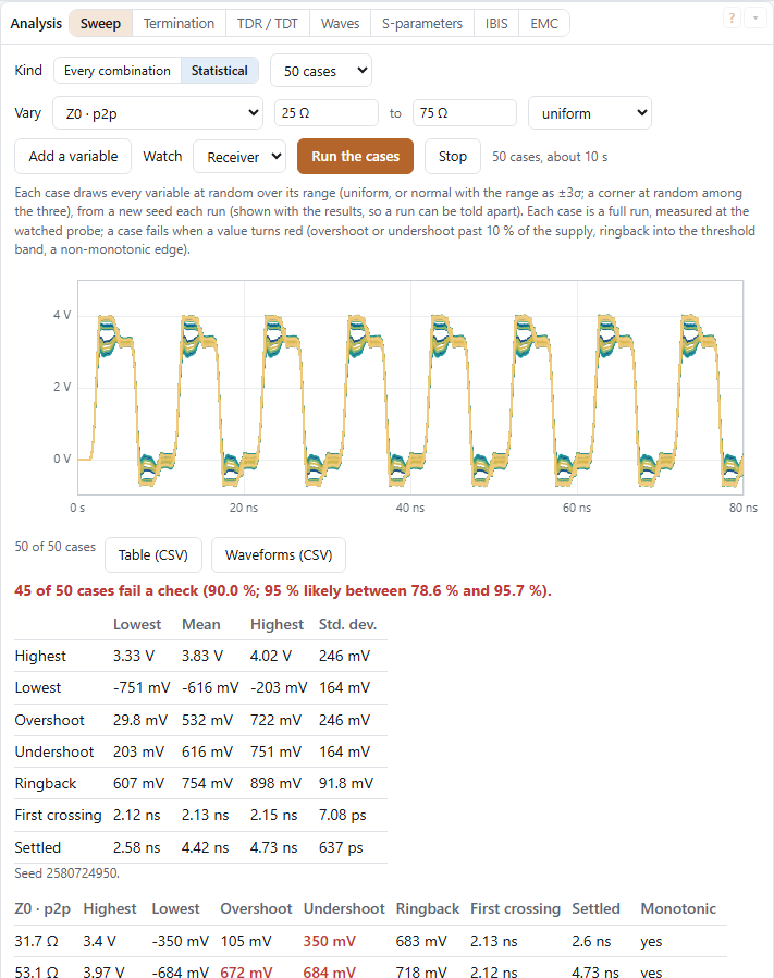
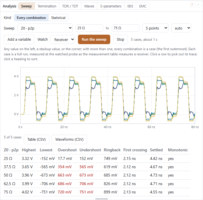
Pick any value on the left (or the corner), a range and the number of points; each point is a full run, and the traces are overlaid from dark (first) to light (last) at the probe you watch. The table gives each point's highest and lowest voltage, its final value and when it first crosses the threshold. A range over a decade is stepped logarithmically.

Termination

In a schematic, choose the driver and a receiver it reaches: the line between them gives the textbook values; series at the driver, parallel, Thevenin or AC at the receiver (or a resistor across a differential receiver) are each tried at five values; every receiver the driver reaches is scored. Use draws the termination next to its pin (moving the driver back to make room for a series resistor) and checks that the drawing joins exactly what it should; where there is no room, it says so and gives the values to place by hand.

For the point-to-point, daisy-chain, star and source-synchronous topologies: each kind of termination starts from its textbook value and is then simulated at five values around it, and the best of each is listed.

• Series: Z0 minus the driver's output impedance, from the slope of its pull-down I-V table near 0 V.
• Parallel: Z0 to half the supply. Thevenin: 2·Z0 up and 2·Z0 down (Z0 at half the supply).
• AC: Z0 with a capacitor whose time constant is three round trips of the line.

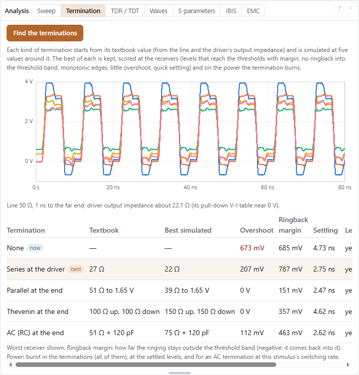
Each run is scored at the worst receiver: levels that miss the thresholds, ringback into the band and a noise margin under a tenth of the supply cost most, then non-monotonic edges, overshoot and settling, and finally the power the terminations burn (an AC termination's from how often the stimulus switches). Use puts a row's values into the topology. Values are standard parts (E24 resistors, E12 capacitors). On a differential pair the view gives the pair's differential impedance to put across the receiver.

IBIS

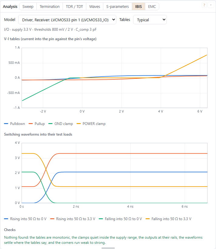
A model in use: its V-I tables against the pin's voltage (pull-up and power clamp turned from the supply to the pin), its switching waveforms into their test loads, at the typical, min or max corner, and checks of its data: tables that turn back on themselves; clamps that carry current inside the supply range (counted twice when they repeat the pull-up or pull-down); an output that does not settle at its rail (normal for offset drivers such as LVDS-like ones, so only a note); waveforms that end where the V-I tables would not put them into the same load; and corners out of order. Nothing found means the data is self-consistent, not that the model matches its silicon.

EMC

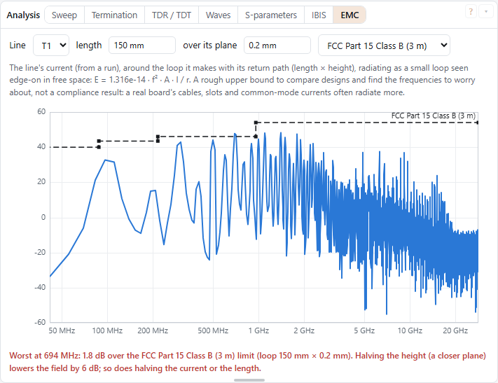
A first estimate of what a line radiates: the line's current (from a run) around the loop it makes with its return under it (length × height over its plane, the height from the stackup for a line by geometry), radiating as a small loop seen edge-on in free space, E = 1.316·10⁻¹⁴ · f² · A · I / r, against the FCC Part 15 or CISPR 32 class A or B limit at that limit's distance. The plot and the worst margin show which frequencies to worry about and how designs compare; it is an upper bound for the line alone and no compliance result: cables, slots in the planes and common-mode currents often radiate more. Halving the height, the current or the length lowers the field by 6 dB.

TDR / TDT

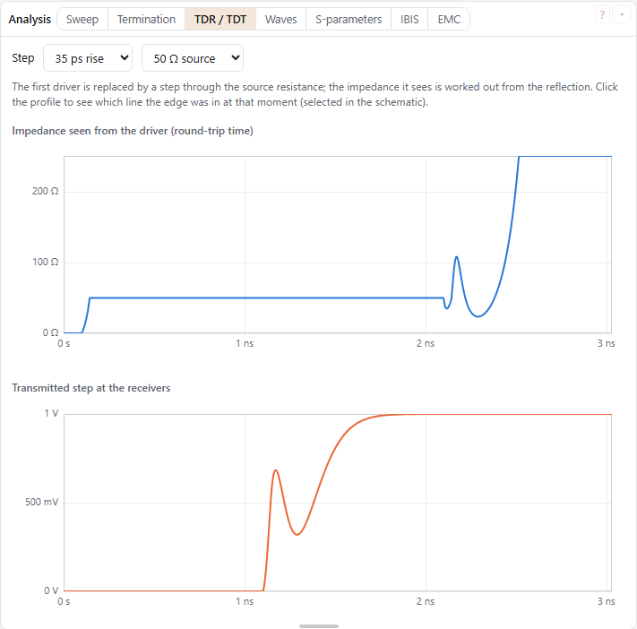
The first driver is replaced by a step through a source resistance (25–100 Ω) with a rise time of your choice. The reflection gives the impedance the step sees along the way, plotted against round-trip time, and the receivers show the transmitted step. Click the impedance profile to see which line the edge was in at that moment; in a schematic the line is selected. Past the far end of the lines the impedance runs off to an open circuit; the plot stops there.

Waves

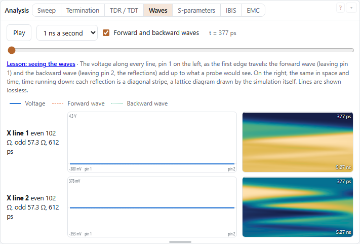
The voltage along every line, from pin 1 on the left to pin 2 on the right, animated as the first edge travels (Play, a speed in nanoseconds per second, or the slider). On a line, the voltage anywhere is a forward wave (leaving pin 1) plus a backward wave (leaving pin 2: the reflections), and both follow from what the run recorded at the two ends. Beside each line, the same voltage in space and time, time running down: every reflection is a diagonal stripe, which is the classic lattice diagram, drawn from the simulation. Lines are shown lossless. Coupled lines (a differential pair, an aggressor and its victim, up to eight lines side by side) are drawn line by line: their modes (for a pair, even and odd) travel apart at their own speeds, each like a single line, and every line's voltage is the sum of the modes there, so the crosstalk on a quiet line can be seen travelling along it. A pair driven differentially also gets a differential row (line 1 − line 2). Every row has its own voltage scale (its numbers at the left), so a small swing fills its plot and its space-time picture.

S-parameters and ports

Compute solves the passive network (lines, coupled lines, resistors, capacitors, inductors) at every frequency from DC up to the frequency given, and gives a Touchstone 2 file with a 50 Ω reference. Lines use their own models (lossy unless Lines is set to Ideal), not a fit, and are solved in a wave form that stays exact at their resonances. Open in the S-parameters tab adds the result to the S-parameter tool, ready for its plots, quality checks and time domain; Download saves the file.

• Ports: in a schematic, Port parts (from the parts list) are the ports, by their number, each to ground with its reference impedance. In a run a port is that impedance to ground, like an instrument.
• Without Port parts, every driver and receiver pin becomes a port, drivers first; a differential buffer gives two (+ and −). Buffers and their packages are not part of the network.

Coupled lines and crosstalk

Lines close together share their field: an edge on one line couples onto its neighbours. In a schematic, the Coupled part holds two to eight lines side by side. Define it by its geometry on the design's stackup (layer, width, spacing and length), or a pair by its even and odd impedances and delays. Pins 1 to n are the near ends of the lines, n + 1 to 2n their far ends.

A pair by geometry can be broadside: one trace on each of two signal layers between the same two planes, offset sideways by the distance you give (0: one over the other). Stacked traces couple more strongly than traces side by side at the same distance.

• Copper splits the bundle into its modes: for a pair, the odd mode (the lines driven against each other) and the even mode (driven together). Each mode has its own impedance and speed. In a mixed dielectric, such as a microstrip half in air, the modes travel at different speeds, and that is what makes far-end crosstalk.
• Lines by geometry are lossy like single lines, each mode with its own loss (the odd mode loses a little more: its current crowds into the inner edges).
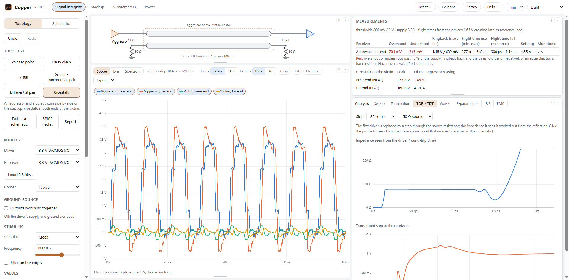
• The Crosstalk topology drives the aggressor and lets the victim rest in a resistance at both ends. The measurements give the victim's peak at its near end (NEXT) and far end (FEXT), as a share of the aggressor's swing. Sweep the spacing runs one edge at seven spacings, from half the trace width to four times it, and lists the crosstalk for each; click a row to use that spacing.

Differential pairs

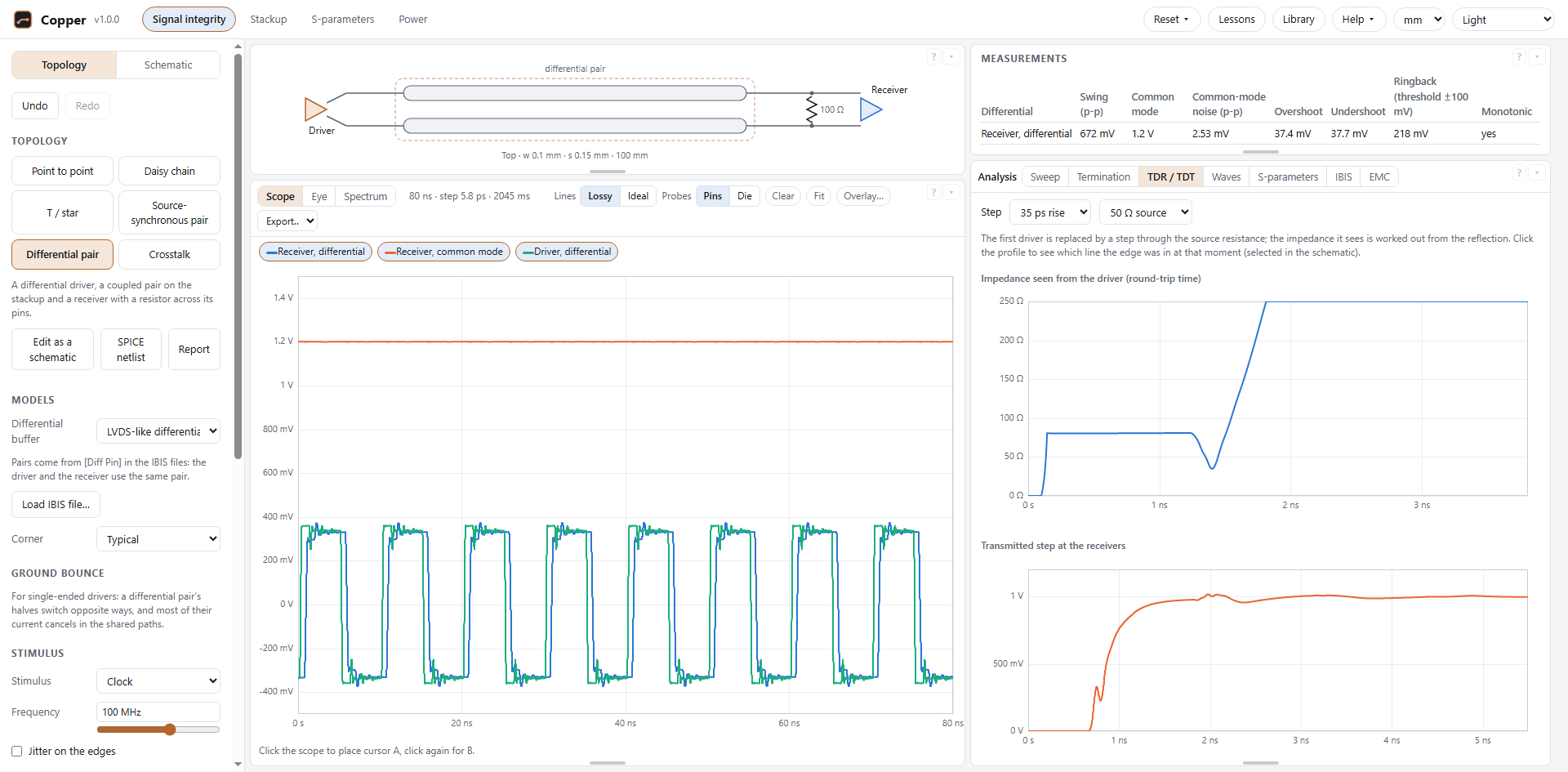
A differential buffer drives two pins in opposite directions, and its receiver reads the difference between them. IBIS files describe such pairs with [Diff Pin]: Copper reads it, and lists each pair under Differential buffer in the Differential pair topology. In a schematic, a driver or receiver with an inverting pin has two pins: + (pin 1) and − (pin 2). The built-in models include a generic LVDS-like pair: about 340 mV across 100 Ω, around 1.2 V.

• The scope shows the differential voltage (+ minus −), the common mode (their average) and the driver's own differential voltage. In a schematic, the probe U2.1-U2.2 is a difference and U2.1~U2.2 a common mode; tick them for a selected differential buffer.
• The measurements give the swing, the common mode and its noise, overshoot, undershoot and ringback against the receiver's own threshold (± its [Diff Pin] vdiff; 100 mV when the file gives none).

More parts: blocks, vias, beads, connectors, packages, cables, current sources

S-parameter blocks

A block puts a network from a Touchstone file (or CITI, or a table) into a schematic: port k is pin k, against ground. Add one with S-param in the parts list, or with To schematic on a file in the S-parameters tab. The file's data is stored in the design: it goes with the design, into design files, and into links when it is small (larger ones: share the design file).

• In a run, each term is fitted once: a rational function with its delay taken out where that fits within half a percent, otherwise the term's impulse response (the data flat to 60 % of its top frequency, tapered to zero at the top). A matrix that gains more than half a percent anywhere is scaled down to be passive, with a note.
• When the data stops below the fastest edge's knee (0.35 divided by its rise time), the run goes ahead with a note: edges through the block come out slower than they would.
• The block's panel shows the file's ports and frequency range, and how its terms ran. In S-parameter results (Analysis), a block uses its own data inside its band.

Vias

A Via goes from one copper layer of the design's stackup to another, with its drill, pad and antipad. Its barrel is worked out as a short coaxial line in the board: capacitance to the planes' antipad edges, inductance to its return (the antipad, or a return via at the distance you give), and the dielectric it passes. Its pads add their capacitance; the barrel beyond the layers it joins is a stub to the board's outer layers, which backdrilling cuts to a residual length. Non-functional pads on the unused signal layers add theirs. The panel gives the barrel's impedance and delay, the pad capacitance, and the stub's quarter-wave frequency, where the through path dips (lower in practice, with its pads).

The via is an estimate, good for the barrel's delay and a stub's notch to about 10 % when return vias are within about 1 mm of it; with a large antipad and distant return vias the real via is slower and its notch lower (by up to about 20 %). For a via that decides a design, use its S-parameters from a 3D field solver in a block.

Unused pad (under Non-functional pads) gives the pads on unused layers their own diameter, often smaller than the connected pads: they load the barrel less.

A Diff via is two vias of the same make, their centres a pitch apart, in one antipad round both (its width the pitch plus the antipad). Each stretch of barrel is a coupled pair: the two barrels inside the antipad as two wires in a round shield (the circle round the opening), which gives their odd and even impedances (Zdiff = 120/√εr · ln((2p/d)(1 − σ²)/(1 + σ²)), σ the pitch over the antipad's width). Pins 1 and 2 are the P and N vias on the From layer, 3 and 4 on the To layer. Stretches shorter than 2 ps run as two single vias. Like the single via, an estimate.

The point-to-point and daisy-chain topologies can have vias at the driver and the receivers: down to the line's layer at the driver, and back up at each receiver, on the topology's stackup.

Ferrite beads, connectors and packages

• Ferrite bead: its impedance at 100 MHz, its DC resistance, and its peak (impedance and frequency), as a DC resistance in series with a parallel R-L-C. Generic presets are named by their values.
• Connector: a short line (Z0 and delay) with each pin's inductance and capacitance at both ends; presets for a few common kinds. A connector with coupling between its pins is better as its S-parameter file in a block.
• Package: R, L and C between a buffer (pin 1) and the board (pin 2), half the capacitance at each end.

Cables

A Cable is coax (inner diameter d, the shield's inner diameter D) or a round wire over a plane (diameter d, its centre at height h); a Cable pair is twin lead or a twisted pair (wires d, centres s apart, and optionally the height of the pair over a plane or shield). They follow the closed forms in one dielectric (give its effective εr, counting the jacket and air): Z0 = 60/√εr · ln(D/d) for coax, 60/√εr · acosh(2h/d) for a wire over a plane, Zdiff = 120/√εr · acosh(s/d) for a pair. A twist lengthens the wire by its factor. Their loss is solid copper's skin effect (with the current crowding towards the return) and the dielectric's loss tangent: a braided shield or stranded wire loses more. A cable runs as a lossy line, a pair as a lossy coupled pair (pins like a coupled pair's). Presets give common sizes; save your own in your library.

Current sources

A Current source pushes current out of its pin 1 into the circuit and back into pin 2, following the stimulus from its low (0 A) to its high, or its own points. It is ideal (no resistance across it), so it is open in S-parameters. For a load drawing current from a node, put pin 2 on the node and pin 1 on ground.