S-parameters

Getting started

1. Choose Open files…, drop files anywhere on the page, or pick one from Examples (or from the buttons in an empty plot). On a first visit an example is open already.
2. The first two plots show the main through path and the input reflection. For a file with differential pairs that is SDD21 and SDD11.
3. Click a plot to make it active (it gets an outline), then click terms in the Terms matrix to add or remove them.
4. Everything you change can be undone with Undo or Ctrl+Z.

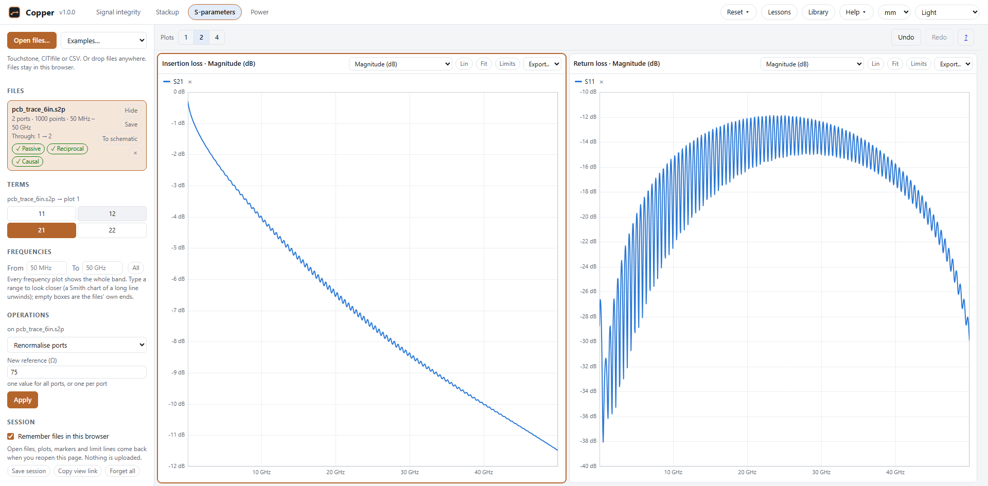
The examples are made-up channels, for trying the tool. They are not reference data.

Files

Copper reads these formats:

• Touchstone 1.x and 2.x (.s1p to .s32p, .ts): every data format (RI, MA, DB) and every parameter type (S, Y, Z, H, G; all are converted to S). Version 2 files may use upper or lower triangles, any port order, per-port reference impedances and mixed-mode order.
• CITIfile (.cti, .citi): each data package becomes its own network. Terms missing from the file show as gaps.
• CSV and TSV tables: a frequency column and columns of dB, magnitude and phase, or real and imaginary parts. The column mapping is guessed from the headers and reported in a message.

Each file in the list shows its ports, points and frequency range, how its ports were paired, and three quality badges (see Quality checks). Its buttons hide or show it in every plot, save it as Touchstone (Save) and close it (×). Each file keeps one colour in every plot.

Pairing. Ports are paired automatically: odd-even (1-2, 3-4…) or side by side (1 to N/2 on one side), with the polarity of each pair checked from the low-frequency data. The result is shown under the file name.

Terms

The matrix shows the terms of the selected file for the active plot. A highlighted cell is shown in that plot; click it to add or remove it.

• Single-ended terms Sij for every port pair.
• Mixed mode (files with pairs): differential (SDD), common-mode (SCC) and mode-conversion (SDC, SCD) terms, computed from the single-ended data.
• Shift+click a term to add it for every open file that has it, or to remove it from all of them.

Plots

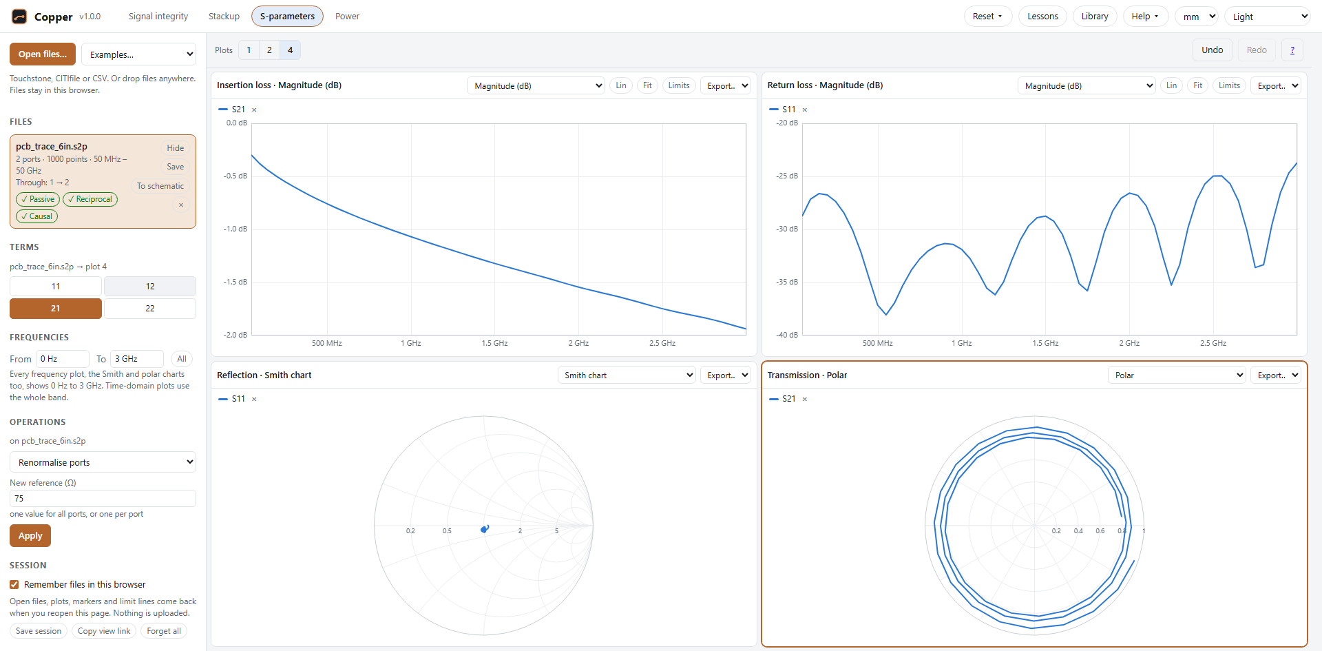
Show 1, 2 or 4 plots with the buttons above them. Each plot has its own type:

• Magnitude in dB or linear, phase (wrapped or unwrapped) and group delay, against frequency (Lin/Log switches the axis);
• Smith chart and polar chart;
• the time-domain responses (see Time domain) and the quality plots (see Quality checks).

Hover to read values. Drag a box to zoom, Shift+drag (or drag with the right button) to pan, Ctrl+wheel to zoom the frequency axis around the pointer; Fit (on the plot's bar) or a double-click shows all of it again. The mouse wheel alone scrolls the page. Export… saves the plot as PNG or SVG, or its data as CSV.

Frequencies, on the left, sets the band every frequency plot shows, the Smith and polar charts too: From and To (empty: the open files’ own ends), or All again. Group delay is worked out over the whole band first, so a narrow band doesn’t change it. Time-domain plots always use the whole band, which they need. A view link carries the band.

A Smith chart reads impedance from a reflection (S11, S22). A transmission term such as S21 can be drawn on it, but it has no impedance there; polar shows the same points without the grid, and the plot says so. A long line winds S21 once round for every 1 / delay of frequency (a 1 ns line: once per GHz), so over a wide band its trace is a tight spiral: a narrower band under Frequencies unwinds it.

Markers and limit lines

Markers. Click a plot to place a marker (up to six per plot). The table under the plot reads every trace at each marker; × removes one.

Limit lines. Limits opens the plot's limit lines. Each line is an upper or lower limit through points you type in (frequency and value) or draw: press Draw and click the plot. Between points the line is straight on the plot's axes. The legend shows a verdict for every trace: ✓ when it stays on the right side, ✗ with the worst violation and where it happens.

Quality checks

Every file is checked with the frequency-domain quality metrics of IEEE Std 370-2020. Each badge gives a level: good, acceptable, inconclusive or poor. Click a badge to put its plot in the active plot, showing where in frequency the problems are.

• Passivity: a passive network can't give out more power than it receives, so the largest singular value of S must not exceed 1. The plot shows it against frequency with the limit.
• Reciprocity: for a passive linear network Sij = Sji. The plot shows the mean difference in dB.
• Causality: a causal response turns clockwise in the complex plane as frequency rises. The plot shows the share of clockwise rotation for the worst term. A term that never changes (an exact zero in an ideal model) carries no causality information and is left out.

Time domain

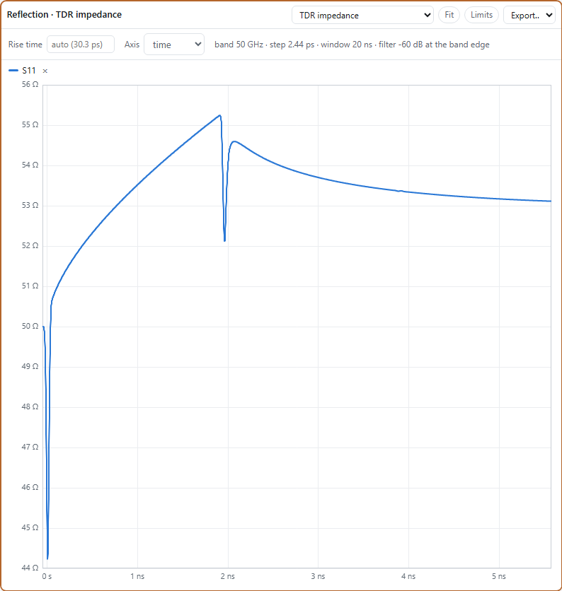
Choose TDR impedance, Step, Impulse or Pulse response as the plot type. The data is put on a uniform frequency grid, extended down to DC, band-limited with a Gaussian filter and transformed with an inverse FFT.

• Rise time: leave it empty for the shortest the data supports (the filter is 60 dB down at the highest frequency), or type one in, such as 35 ps.
• Pulse width applies to the pulse response.
• TDR shows the impedance seen from a port: Z = Z_ref(1 + ρ)/(1 − ρ). For differential terms the reference is twice the port impedance; for common-mode terms, half.
• Axis (TDR): time, or distance along the line. Distance is the round trip halved, x = t·c / (2√ε_eff), with ε_eff the line's effective relative permittivity (about 4 for a stripline in FR-4, about 3 for a microstrip). Markers and limit lines move with the axis.

The row above the plot shows the band, the time step, the window and the filter level at the band edge, with a warning when the data limits the result (for example a rise time shorter than the bandwidth allows).

Operations

Operations work on the selected file and add their result as a new file, tagged result. Results can be viewed, checked, used in further operations and saved as Touchstone.

• Renormalise ports to a new reference impedance (one value, or one per port).
• Terminate ports in a load (a value, open or short), leaving the other ports.
• Reorder ports: give the new order, each port once.
• To mixed mode: a file of differential and common-mode ports, using the pairs found.
• Cascade with another file, its port 2 (or right side) to the next file's port 1 (or left side).
• De-embed fixtures: remove a left fixture and a right one (or the left one mirrored) from a measurement.
• Split a 2x-thru: split the measurement of two fixture halves joined back to back into its left and right halves, for de-embedding. A 2-port is split directly. A 4-port with one differential pair on each side is split per mode (differential and common mode separately); mode conversion in the 2x-thru is reported, not kept. Where the 2x-thru passes almost nothing (below −40 dB, for example at a via stub's resonance), a warning says so: no de-embedding can see through the fixture there.

For 4-port and larger files you choose how ports are numbered: side by side (1 to N/2 on the left) or odd-even (odd ports on the left).

Sessions and sharing

• Remember files in this browser (on by default): your files, plots, markers and limit lines come back when you reopen the page. They are stored only in this browser. Turn it off to keep nothing; what was stored is deleted.
• Save session writes the files and the view into one .json file. Open it with Open files… to get everything back; Undo returns to what was open before.
• Copy view link copies a link that carries the layout, plot types, axes, time-domain settings, markers and limit lines, but no files or data. Someone who opens it sees their own files the same way.
• Forget all closes every file and deletes what this browser has stored. Click it twice to confirm.