Stackup
The board’s layers, and the impedance, delay and loss of a trace or a pair worked out from its geometry by a field solver, with a picture of the field. Signal integrity uses this board for its vias and for every line set by geometry.
Stackup and line impedance
The Stackup tab edits the layers of the board: signal layers (copper with traces), planes (solid copper) and
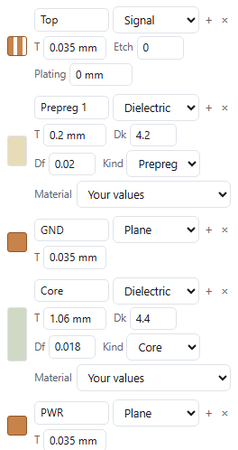
dielectrics (core or prepreg, with their Dk and Df), from the top down, plus solder mask and the etch factor. Each
design has its own stackup, saved with it (in its file and its link); the ready-made topologies have one too. Start
from a 2-, 4-, 6- or 8-layer starter and change it: type values with units (0.1 mm, 4 mil,
35um) or scroll over them. Undo and Redo at the top of the sidebar (or Ctrl+Z and Ctrl+Shift+Z)
work here as everywhere. The board is the one Signal integrity uses: its vias and every line set by geometry are worked
out from these layers, so a change here changes the scope there.
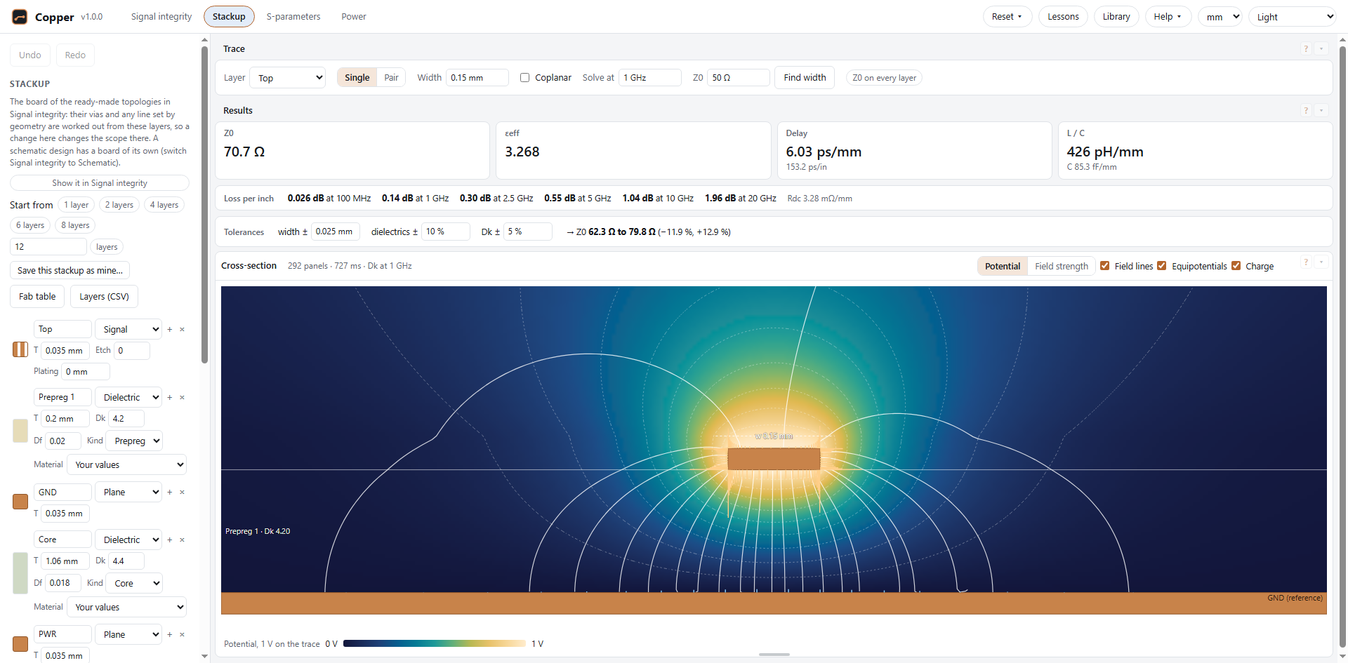
Above the cross-section, choose a signal layer, a single trace or a pair, the width (and spacing), and Copper solves it as you change anything: Z0, εeff, the delay per mm and per inch, and L and C per mm; for a pair the differential and common impedances and the odd and even modes. Find width gives the width for a target impedance.
- The nearest plane above and below a trace are its references; layers beyond them don't matter. An outer trace sits on the board under the mask; an inner one is surrounded by the prepreg beside it.
- The solder mask can be on both sides, on the top or the bottom only, or left off. Each signal layer can have its own etch factor (on its row; the stackup's otherwise), and an outer layer plating, which adds to its traces' thickness.
- Dk and Df are given at one frequency (1 GHz unless you change it) and follow a wideband model of real laminates elsewhere: Dk falls slowly as the frequency rises. Solve at picks the frequency for the impedance.
- The solver works on the cross-section's boundaries (traces, planes, every dielectric interface) and is checked against exact results for stripline and coupled stripline and against published microstrip formulas, within a few tenths of a percent, and for coplanar lines against an independent finite-difference solution, within 0.1 %.
Lines by geometry: in a schematic, select a transmission line and set Defined by to Geometry on the stackup; give it a layer, a width and a length. Copper works out its Z0 and delay from the design's stackup when the net runs and shows them under the line. Change the stackup and the net changes with it.
For a pair, Find spacing keeps the width and finds the spacing that gives the target Zdiff (it says so when the target is out of reach at that width). Z0 on every layer (or Zdiff on every layer) switches on a table of the impedance, delay and effective permittivity of the current trace on each signal layer, kept up to date with every change until you switch it off. Save this stackup as mine keeps it in your library (see Your library).
Any number of copper layers from 1 to 180 (the most any PCB maker has built): type the number next to the starters and press layers for a board with signal layers outside and planes and signals alternating inside (every signal layer beside a plane), 1.6 mm up to 10 layers, thicker above (5 mm at 40 to 60 layers, about 15 mm at 180). 2 layers starts a two-layer board: signals on top, a ground plane on the bottom. 1 layer starts a board with copper on one side of a 1.6 mm core and nothing under it: a line there has no plane, so it takes its return from coplanar ground beside it. Every layer can then be changed as usual.
For a pair, Along the line shows a signal launched on one trace at a distance down the pair (move the Along slider): how far its potential swings around each trace. The signal is half the even mode and half the odd one; where they travel at different speeds (microstrip: part of the field is in the air) it moves over to the neighbour and back as the distance grows, and the readout says how far it is to go all the way across at the frequency you give. In stripline the two modes travel together and it stays put: forward crosstalk needs an inhomogeneous line.
Materials
Each dielectric has a Material list of typical laminate classes. Picking one sets the layer's Dk and Df at once; typing your own values shows Your values. The classes are typical figures at about 1 GHz, not any one maker's laminate: use your laminate's data sheet where the last per cent matters.
| Class | Dk | Df | Typical use |
|---|---|---|---|
| FR-4, standard | 4.3 | 0.02 | General boards, edges slower than about 1 ns |
| FR-4, mid loss | 3.9 | 0.01 | A few Gb/s |
| Low loss | 3.6 | 0.006 | 5 to 10 Gb/s |
| Very low loss | 3.4 | 0.003 | 10 to 28 Gb/s, long channels |
| Ultra low loss | 3.1 | 0.0015 | 56 Gb/s and up |
| PTFE ceramic | 3.0 | 0.0012 | RF and microwave |
| Polyimide | 3.3 | 0.004 | Flex and rigid-flex |
Coplanar ground
Coplanar, next to the width, puts ground copper beside the trace on its own layer, a Gap away from each edge (0.15 mm to start). With a plane below as well, the line is a grounded coplanar line: the side grounds pull the field in and lower Z0, more the smaller the gap. On a layer with no plane above or below (the 1-layer board, or a board whose planes you removed) the side grounds are its only return, so the switch is on and can't be turned off.
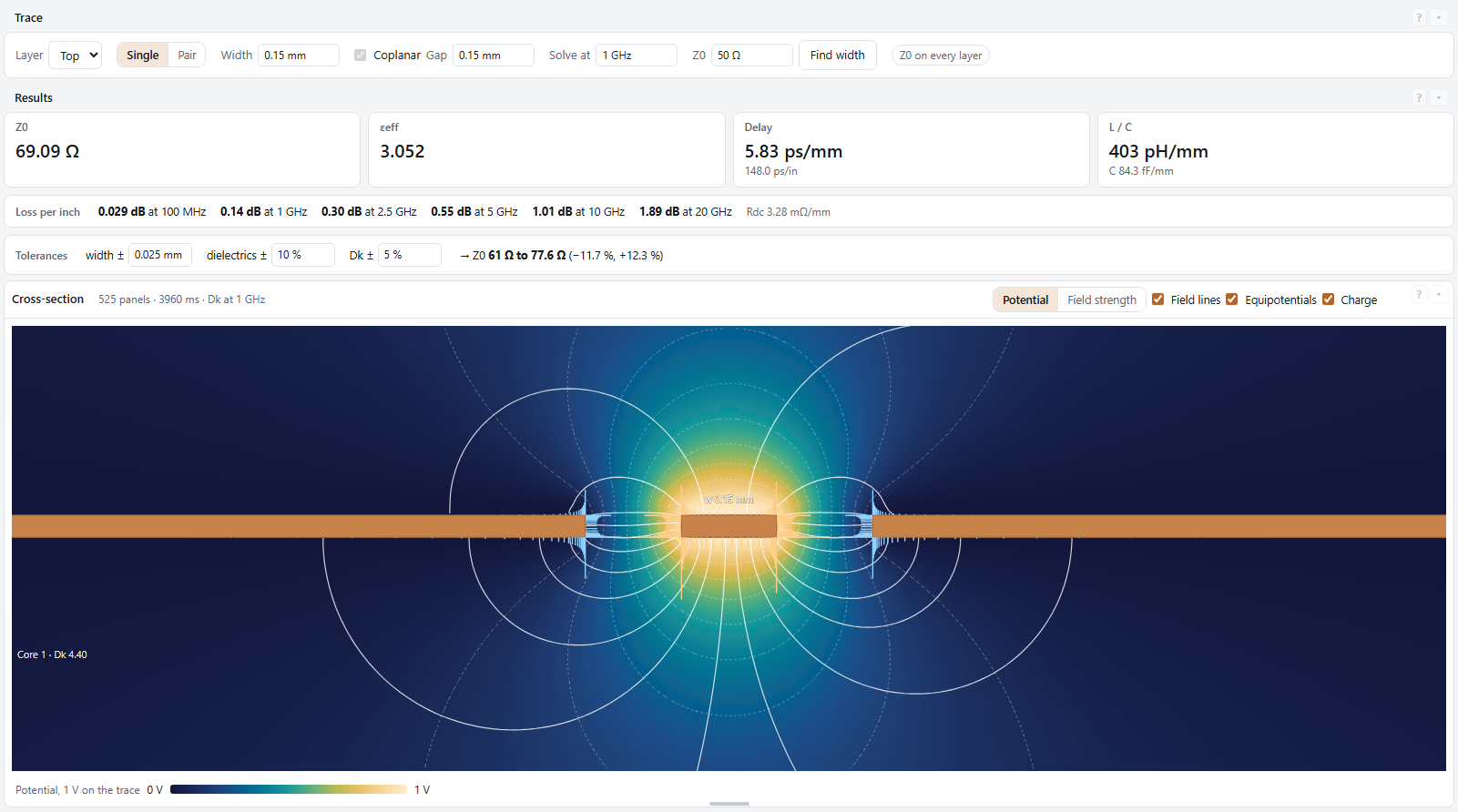
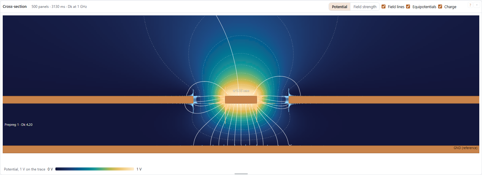
- The side grounds are drawn and solved as copper as thick as the trace and at least ten times as wide as the line and its gaps (more on a thick board); wider changes nothing you would see.
- The picture shows the field ending on them, and their charge.
- In a schematic, a line by geometry has the same Coplanar ground box and gap, so a net can run on a one-layer board.
- Coplanar lines are checked against an independent finite-difference solution, within 0.1 % over thin and thick copper, with and without a plane below.
Fabrication tolerances
A board maker holds the trace width, the dielectric thicknesses and the laminate's Dk only within a tolerance. The Tolerances row under the results gives the range of Z0 (or Zdiff) they allow: width ± (25 µm to start; the gap to a coplanar ground and a pair's spacing open as much as the trace narrows), dielectrics ± (10 %) and Dk ± (5 %). Copper solves the two corners: the high one with the trace narrow, the dielectrics thick and Dk low; the low one the other way round. Every other combination lies between them.

A 50 Ω microstrip on 0.2 mm of FR-4 typically spans about ±10 %: often more than the rounding of the target, and the reason board makers quote impedance control as ±10 %. Narrow traces on thin dielectrics spread the most.
The fab table and the layer file
Fab table saves one page for a board maker or for print: the layers top first (thickness, copper weight, material, Dk and Df), the board's total thickness, the trace you are planning with its impedance and, with the tolerances above, its range, and the cross-section picture. Layers (CSV) saves the same layers as a spreadsheet file (thicknesses in mm and mil, copper in ounces).
The field picture
The cross-section is drawn to scale around the trace (on a thick board, a close-up of the traces: the far plane is left out and named at the edge, with how far away it is), coloured by the potential (1 V on the trace, 0 V on the planes) or by the field strength (on a log scale). For a pair, choose the odd (differential: +1 V and −1 V) or even (common: both at 1 V) mode.
- Field lines start on the trace, spaced by its charge: where they crowd, the field is strong. They end on the other conductors.
- Equipotentials are drawn every tenth of the trace's voltage.
- Charge shows how the charge sits on the conductors: bunched at the trace's edges, and on the plane right under the trace, which is where the return current flows. A trace close to its plane keeps its return current narrow; one far from it spreads it out.
The colour scales are designed to be read in steps of equal brightness, so they also read in grey and with most colour-vision deficiencies.
Lossy lines
Real lines lose signal in their copper and in their dielectric, more at high frequencies than at low ones: edges arrive slower and lower, and a long line rounds them off. Copper simulates that wherever it knows the loss, and the scope's Lines: Lossy | Ideal switch runs everything lossless instead, so the afterglow shows the two side by side.
- Lines by geometry take their loss from the stackup: the copper's resistance at DC and with the skin effect (the current crowding at the trace's edges and on the plane under it included), the roughness of the copper foil, and each dielectric's Df. The Stackup tab shows the loss per inch from 100 MHz to 20 GHz.
- Copper (on the Stackup tab): its resistivity and the foil's roughness by the Huray model, with smooth, HVLP, VLP and standard presets, or your own sphere radius and surface ratio. Rough copper loses up to 1 + ratio times as much as smooth copper at high frequency.
- Lines given as Z0 and delay, in schematics and in the ready-made topologies, can be made lossy: the loss in dB per inch at a frequency, the share of it that is in the copper (the rest is in the dielectric), and the delay per inch, which tells how long a line of a given delay is.
- Copper loss grows with the square root of the frequency and dielectric loss in proportion to it. Both come with the small change of impedance and delay with frequency that goes with them, so the result is causal: nothing arrives before it can.
In the time domain each lossy line is described by its characteristic admittance and its propagation over the line, each fitted with a sum of simple poles (checked to stay within 0.1 dB of the exact line up to three times the fastest edge's knee frequency) and run as recursive convolutions, so a lossy line costs little more than an ideal one. The response is checked against the exact line computed in the frequency domain.
A line given as Z0 and delay can also have a DC resistance (per inch): its copper loss then starts from that resistance at low frequency and joins the √f rise of the skin effect above, as a line by geometry does. (The skin effect never adds to the DC resistance: once the current has moved to the surface, the DC value no longer applies.)